
<문제에서 사용된 csv 파일>

문제1
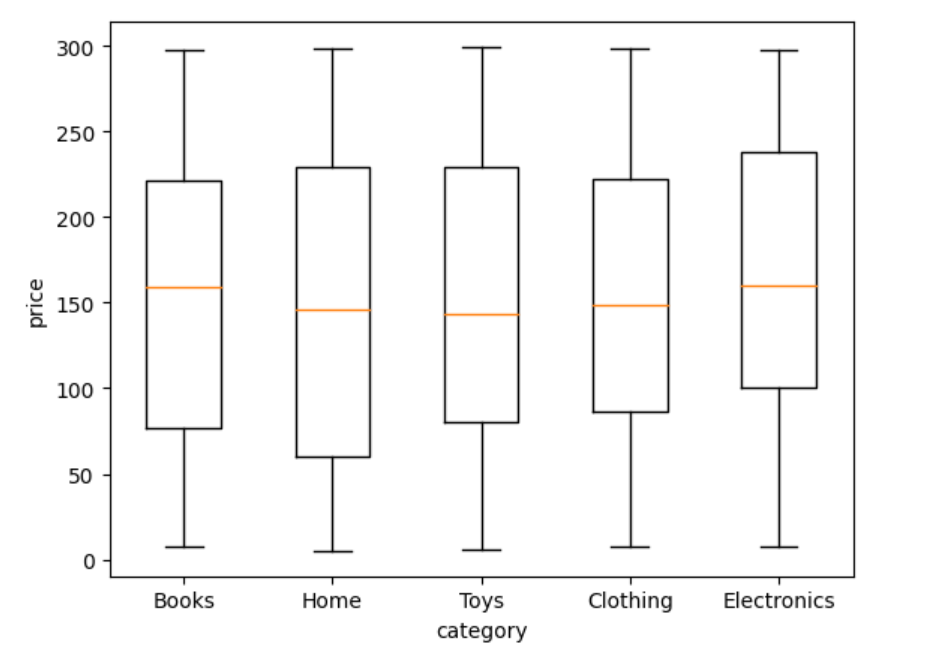
price 컬럼에 대해 제품 가격의 분포를 Box Plot으로 시각화하세요. 카테고리별로 그룹화하여 시각화하세요.
# 내풀이
import matplotlib.pyplot as plt
import pandas as pd
df = pd.read_csv('./user_purchase_data.csv')
category = df['category'].unique()
category_price = [df[df['category']==x]['price'].tolist() for x in category]

# box plot 그리기
plt.boxplot(category_price, labels = category)
plt.ylabel('price')
plt.xlabel('category')
plt.show()
matplotlib을 사용할 때는 결측값을 제거해 주어야 한다.
결측값이 포한된 데이터가 있을 경우 오류를 발생시키거나 박스 플롯을 제대로 그리지 못할 수 있기 때문이다.
처음에 csv 파일을 불러와서 바로 boxplot을 실행시키니까 아무 그림도 그려지지 않았다.
그래서 결측값을 제거해 보니까 첫번째 그림이 나왔고,
앞의 결측값과 이상값을 모두 제거한 df로 그렸을 때는 두번째 그림이 나왔다.

정답
import matplotlib.pyplot as plt
import seaborn as sns

# 데이터 로드
data = pd.read_csv('./user_purchase_data.csv')

# Box Plot 시각화
plt.figure(figsize=(12, 10))
sns.boxplot(x='category', y='price', data=data)
plt.title('Price Distribution by Category')
plt.xticks(rotation=45)
plt.show()
seaborn의 boxplot 함수는 자체적으로 결측값을 제거한 후에 그래프를 그린다!

문제2
age 와 total_spent 컬럼을 이용하여 사용자 나이와 총 지출 금액 간의 관계를 Scatter Plot으로 시각화하세요.
# 내풀이
plt.scatter(df['age'],df['total_spent'])
plt.show()
정답
# 데이터 로드
data = pd.read_csv('./user_purchase_data.csv')

# Scatter Plot 시각화
plt.figure(figsize=(10, 6))
plt.scatter(data['age'], data['total_spent'])
plt.title('Age vs Total Spent')
plt.xlabel('Age')
plt.ylabel('Total Spent')
plt.show()
라벨과 figsize 설정을 추가로 해주었다.

문제3
모든 수치형 데이터 (price, quantity, total_spent, age, ad_spend, visit_duration) 간의 상관관계를 분석하고, heatmap을 사용하여 시각화하세요.
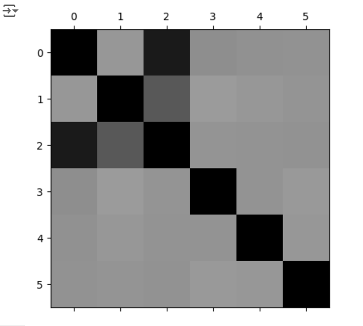
matplotlib을 이용해서 heatmap 그리기
# 내풀이
corr=df[['price','quantity','total_spent','age','ad_spend','visit_duration']].corr()
cmap = plt.get_cmap('Greys')
plt.matshow(corr,cmap=cmap)
plt.clim(-1.0, 1.0)
plt.show()
.corr() 함수를 이용하면 상관관계를 구할 수 있고,
이후 이 값을 plt.matshow()함수에 넣어서 heatmap을 그릴 수 있다.
cmap = plt.get_cmap('Greys') 이 부분은 색을 입히고 싶어서 추가해 주었고,
plt.clim(-1.0, 1.0) 이거는 기본값이 0~1로 되어있는데, 데이터는 상관관계이기 때문에 범위를 -1~1로 지정해주었다.
기본값은 -0.3 의 상관관계가 0과 값이 똑같이 나오기 때문에, 범위를 바꿔줘야 알맞게 시각화를 할 수 있다.
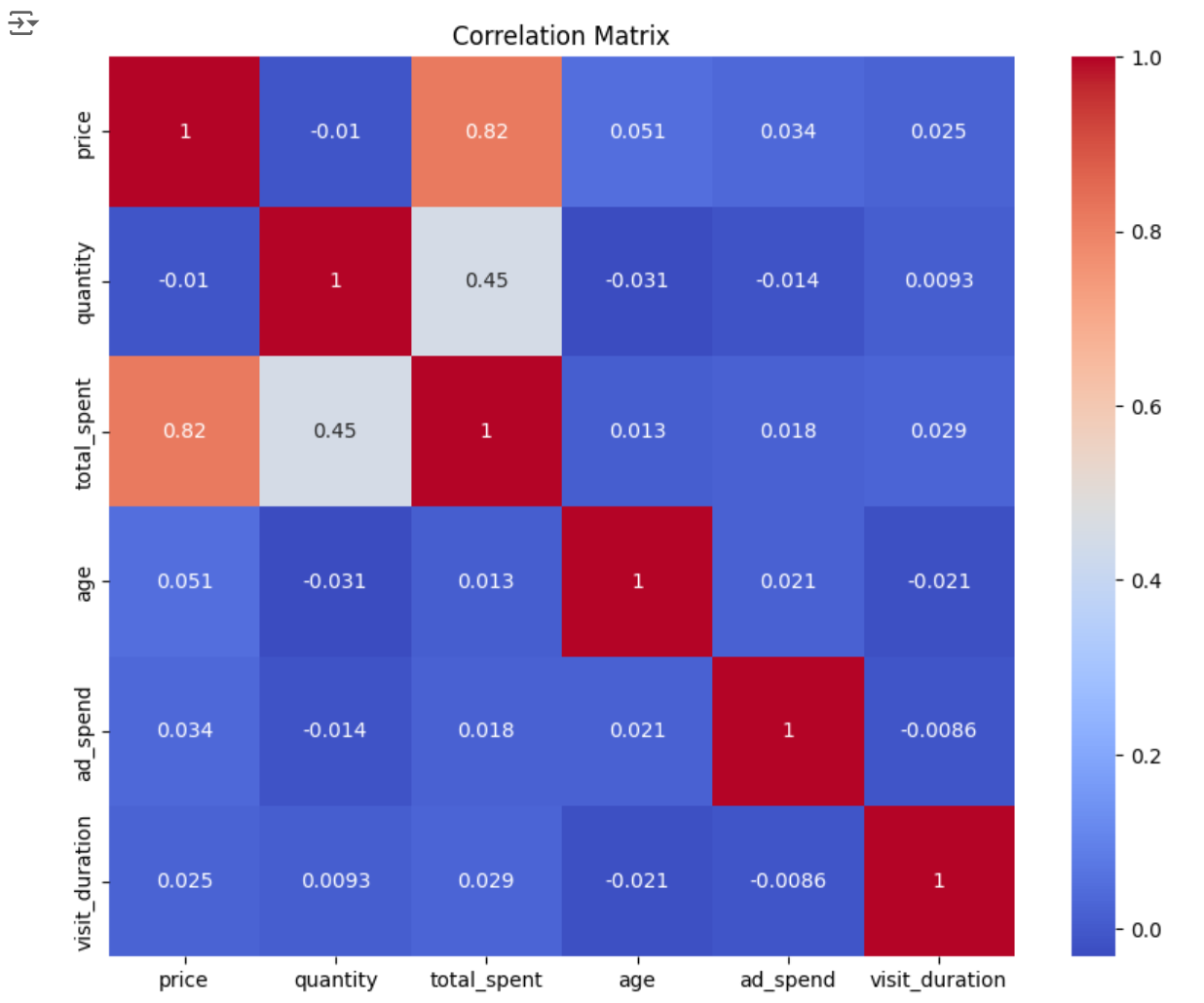
정답 : seaborn으로 heatmap 그리기
# 데이터 로드
data = pd.read_csv('./user_purchase_data.csv')

# 상관관계 분석
correlation_matrix = data[['price', 'quantity', 'total_spent', 'age', 'ad_spend', 'visit_duration']].corr()

# Heatmap 시각화
plt.figure(figsize=(10, 8))
sns.heatmap(correlation_matrix, annot=True, cmap='coolwarm')
plt.title('Correlation Matrix')
plt.show()
아니 seaborn 사용법 아직 안알려줬으면서, 정답은 왜 자꾸 seaborn 사용하는데,,,
seaborn으로는 sns.heatmap()함수를 이용해서 heatmap을 그릴수 있다.
annot =True는 각 셀에 숫자를 보여주고, cmap은 색깔을 지정해 준다.
문제4
age 컬럼에 대한 히스토그램을 작성하여 사용자 나이 분포를 시각화하세요.
# 내풀이
plt.hist(df['age'],bins=40)
plt.xlabel('age')
plt.show()
hist() 함수로 히스토그램을 그릴 수 있으며, bins 파라미터로는 x축의 구간 개수를 지정할 수 있다.

정답
# 데이터 로드
data = pd.read_csv('./user_purchase_data.csv')

# 히스토그램 시각화
plt.figure(figsize=(10, 6))
plt.hist(data['age'], bins=20, edgecolor='k')
plt.title('Age Distribution')
plt.xlabel('Age')
plt.ylabel('Frequency')
plt.show()

문제5
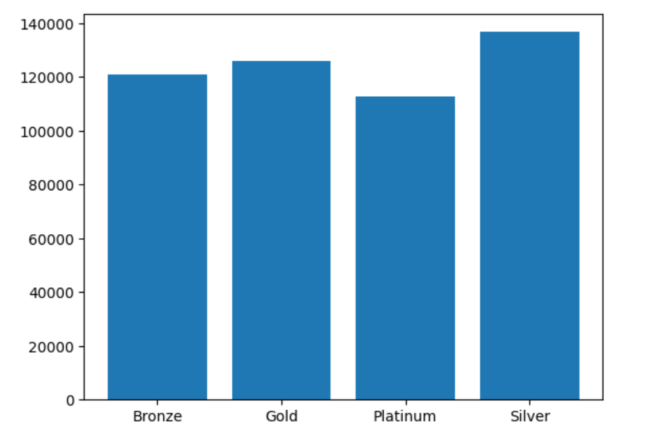
membership_level 컬럼을 사용하여 각 회원 등급별 총 지출 금액을 바 차트로 시각화하세요.
matplotlib으로 막대 그래프 그리기
# 내풀이
membership=sorted(df['membership_level'].unique())
# sorted()를 해 준 이유는 membership_spent와 membership_level 순서를 맞추기 위함
# membership : ['Bronze', 'Gold', 'Platinum', 'Silver']

# membership_level별 total_spent를 별도의 df로 만들기
membership_spent=df[['membership_level','total_spent']].groupby('membership_level').sum()
# 값을 df에서 list로 바꿈
membership_spent=[membership_spent.iloc[x,0] for x in range(4)]

# bar 만들기
plt.bar(membership,membership_spent)
plt.show()
matplotlib은 1차원 array가 들어가야 하기 때문에, 데이터를 전처리 해주어야 한다.
정답 : seaborn으로 막대 그래프 그리기
# 정답
# 데이터 로드
data = pd.read_csv('./user_purchase_data.csv')

# 회원 등급별 총 지출 금액 계산
membership_spent = data.groupby('membership_level')['total_spent'].sum().reset_index()

# 바 차트 시각화
plt.figure(figsize=(10, 6))
sns.barplot(x='membership_level', y='total_spent', data=membership_spent)
plt.title('Total Spent by Membership Level')
plt.xlabel('Membership Level')
plt.ylabel('Total Spent')
plt.show()
seaborn을 이용한 막대 그래프 그리기.
sns는 x, y 파라미터에 df의 컬럼이름을 그대로 가져와서 바로 사용이 가능하며, data에는 데이터프레임 형태가 들어갈 수 있다.

'문제풀이 > 스파르타 - 파이썬 문제' 카테고리의 다른 글
| [Python] 데이터 전처리 & 시각화 | 실습 문제(Pandas) (0) | 2024.07.22 |
|---|---|
| [Python] 파이썬 기초 | 과제 (0) | 2024.07.10 |
| [Python 과제] Lv3. 단어 맞추기 게임 (1) | 2024.05.28 |
| [Python 과제] Lv2. 스파르타 자판기 (0) | 2024.05.27 |
| [Python 과제] Lv1. 랜덤 닉네임 생성기 (0) | 2024.05.24 |